Data
Machining & Machine Learning
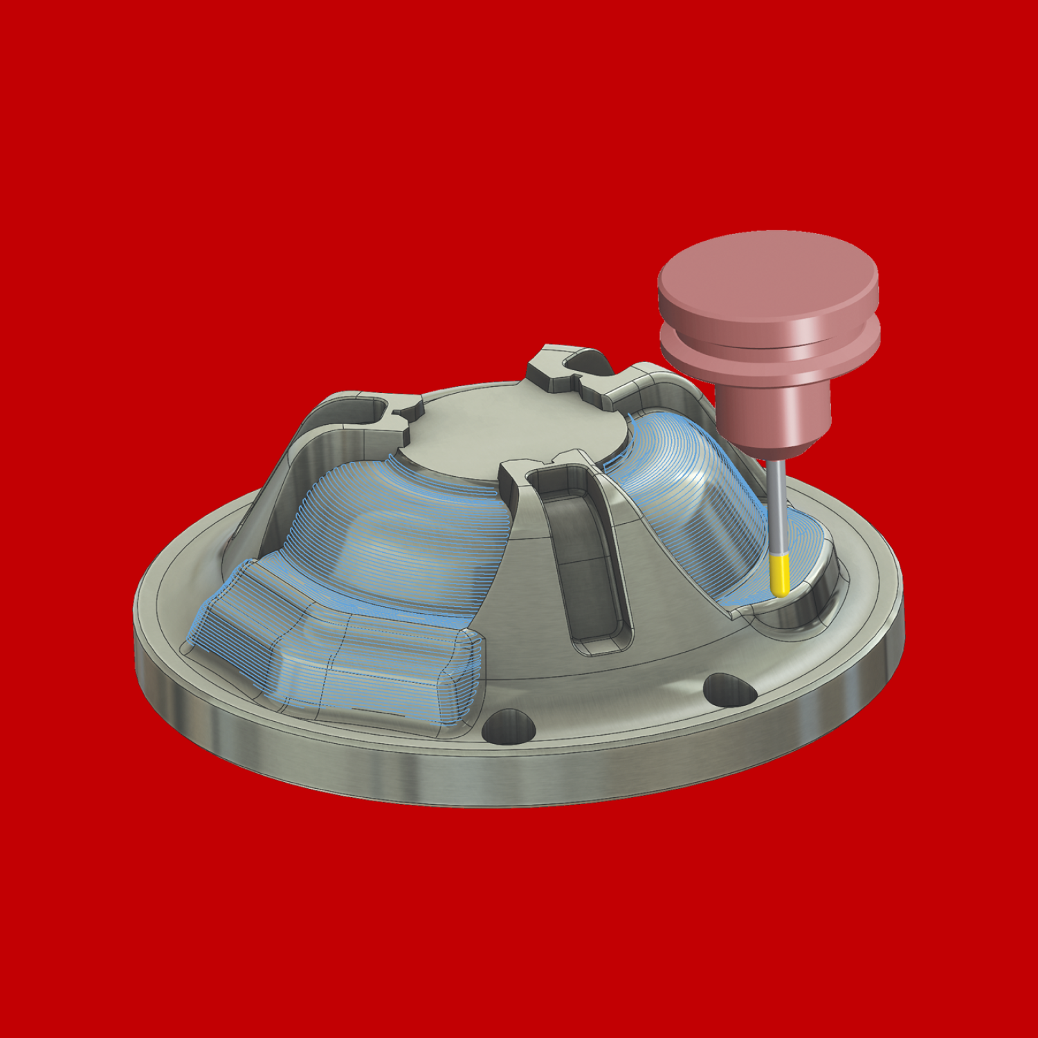
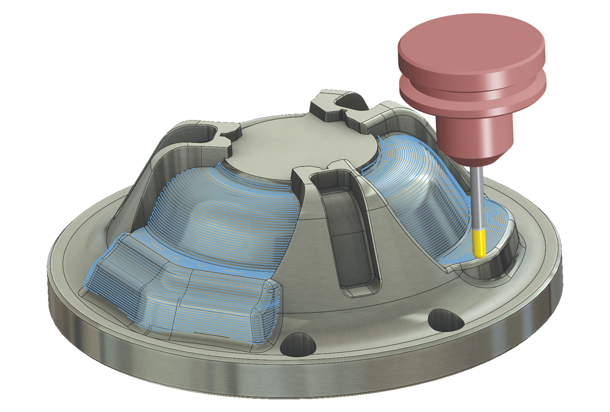
Predict visual inspection outcome by modeling cutting toolpaths from a CNC mill.
Data ━ 22 Oct, 2020
University of Michigan conducted a series of machining experiments on a block of wax measuring 2in x 2in x 1.5in on a Computer Numerically Controlled (CNC) Vertical Milling testbed. The experiments varied feed-rate, clamping pressure and tool condition as it operated with the same program over the 18 experiments. At 100ms intervals, the machining testbed (SMART) recorded 48 features as the tool engraved an S into a block of wax. After the machine finished running the program, both tool and wax underwent a visual inspection to assess tool quality and successful engraving. Our goal is to predict tool condition by modeling the data from these experiments.
Considerations have to be made when trying to assess the majority numerical data within the 18 files, the most important being how a vertical machine operates. Our goal is to predict tool condition and any observations where the tool is not actively cutting, is noise in our model. Many programs found in a large majority of machine shops maintain a typical approach and departure; starting at the machine’s (0,0,0) point located at the extent of each axis, traveling to the part and retracting to a safe plane clear above the part (one would hope!). Both of these tool movement realms are not known for contributing to tool wear and must be removed from consideration by the model.
At each recording interval, both commanded and actual position of all four axis—X, Y, Z and Spindle. The spindle observation consisted of angular snapshots between 0° (or 360°) to 359° and was removed to avoid leakage. Plotting the three axis actual recorded position (X, Y, Z) in a 3D plot will allow better visualization of tool movement and assist in selecting the Z-plane where cutting occurs. The figure below shows one of the 18 experiments actual position plotted, where Z represents height above the work area.
Each layer was named depending on where the program was when the recoding occurred. Selecting a Z plane at 29.5mm will provide the most stringent filter to consider only observations where the tool is in direct contact with the wax. Applying that mask and plotting the resultant actual positions, in the figure below, shows us only the cutting moves that’ll be used for modeling.
Visit the Jupyter Notebook on Github for all the other sanitizing steps taken.
All the moves represented in the plot lie within the space of the block; confirming only observations of interest are present relative to tool wear. Applying this cleaning process to all the other experiments and joining those values with the result of visual inspection and tool wear into one large data set that will be used for modeling.
Another method used for cleaning, was to create a Correlation Matrix to observe any outlier features (like spindle position or command positions) where consistently low correlation was observed.
Almost ready for takeoff, before evoking our predictive model with the cleaned data, weight of our classification bias must be addressed to select adequate baseline metrics. The target for modeling is categorical and there is an imbalance in observations that passed visual inspection. Of the 11,166 recordings, 13.7% failed visual inspection. Due to the imbalance, F1-Scores and Confusion Matrix will be used to evaluate model performance.
Given a classification problem, our baseline will be the most common occurrence of our target—passing visual inspection—at a passing rate of ~86.34%.
Data was piped into a one hot encoder to encode the categorical data and then processed with logistic regression and tuned to have a solution that fits the data, resulting in a test score of 96.37%. An improvement from the basic baseline value! Let’s dig deeper by observing the confusion matrix from this model.
This model is precise in correctly predicting the target, with the incorrect predictions (324) in the hundreds versus the thousands of correct predictions (8,609). The table below with the F1-scores from this model also show high recall and precision around 96.3%.
| no | yes | accuracy | macro avg | weighted avg | |
|---|---|---|---|---|---|
| precision | 0.859761 | 0.980724 | 0.96373 | 0.920243 | 0.964109 |
| recall | 0.879381 | 0.977161 | 0.96373 | 0.928271 | 0.96373 |
| f1-score | 0.86946 | 0.978939 | 0.96373 | 0.9242 | 0.963902 |
| support | 1227 | 7706 | 0.96373 | 8933 | 8933 |
Using both K-Best and a one hot encoder in the random forest classifier model, the model exceeded baseline with a test score of ~96.56% and logistic model score. With such a small improvement, still our best approach for understanding our model is to look at the confusion matrix (the irony!).
The small improvement in our score equates to correct predictions numbering 8,626 and incorrect predictions at 307. Looking at the F1-scores from this model also show an overall improvement averaging out to roughly 96.6%.
| no | yes | accuracy | macro avg | weighted avg | |
|---|---|---|---|---|---|
| precision | 0.863349 | 0.982522 | 0.965633 | 0.922936 | 0.966153 |
| recall | 0.890791 | 0.97755 | 0.965633 | 0.93417 | 0.965633 |
| f1-score | 0.876855 | 0.98003 | 0.965633 | 0.928443 | 0.965858 |
| support | 1227 | 7706 | 0.965633 | 8933 | 8933 |
Using KBest set at 5, our pipeline computed the five most important features when building the model.
The most surprising finding is how important the X axis is to the process. There may be some bias—most of the machining movement occurs in the X direction—in the data; although the graph above sheds some light into another area of investigation—the electrical dimension.
Are the results too good to be true? That may be the case—without more data—how truly effective this model is, whether it was over-fit to the problem, is up for debate. Within this strict data set, these two models look promising and the approach taken to process the data is applicable to other problems within this field. A tantalizing area for more exploration would be to focus on the electrical readings. Feature engineer the electrical data to get an accurate load on the spindle axis may be an important—overlooked in this endeavor—feature to estimate tool wear based on the notion that a dull knife requires more force (electrical energy) to cut (maintain).
Predict visual inspection outcome by modeling cutting toolpaths from a CNC mill.


Extracting actionable data from Immigration Court documents using OCR and Python.